
TrueInsight
Siemens/Altair Channel Partner
Menu


Training a Neural Network in Altair Compose
Check out this blog post to see how you can train a neural network, simply with intuitive software tools.
The world of engineering is ever-changing, with various fields being created and merged daily. In this rapidly changing environment, artificial intelligence (AI) has become a very popular phrase, with many leaders pushing for AI in more and more professions, and engineers are not immune to these changes. This can seem like a daunting “buzzword,” but Altair Compose comes with the tools you need to stay at the edge of innovation. I would like to introduce you to romAI, a powerful pre-packaged neural network designer, trainer, and tester built within Compose behind an easy-to-use GUI. All we need to get started with romAI is a suitable dataset, and then we can be well on our way to creating a custom neural network for whatever task is at hand.
Before diving into this example, I just want to go over a brief explanation of neural networks in case this content is entirely new to you. At its core, a neural network is a complex array of multipliers (or weights) that accept at least one input and provide at least one output. Before training a network, it would most likely give you random outputs, and it would be of little use. We can train it, however, by “showing” it a large set of data with known inputs and outputs, causing those multipliers to adjust with each new piece of training data. If we repeat this process enough times, while also validating that the changes to the multipliers are in fact improving the “knowledge” of the model, we will eventually be left with a structure that can take an input from the training data and give us an output very close to the known output of the training data. Once we are satisfied with its ability to correctly “predict” outputs on data it has already “seen,” we can start showing it data that is new to the model. If everything went according to plan, it should be able to also provide a prediction that is very close to the known output; if this is not the case, then we go back, adjust the model, and train again. Once we are satisfied at this stage, we can use the model in the real world to predict the outputs of complex systems.
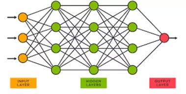
Fig 1. General structure of a neural network.
Figure 1 above shows the general outline of a neural network. The input layer and output layer are fairly self-explanatory, as that is where the inputs and outputs of our data are located, respectively. The green circles represent the “hidden layers,” called so simply because they are not visible as inputs or outputs; this is the part of the model that is trained (the weights). We can adjust these layers in an infinite number of ways, including changing the number of nodes per layer, the number of layers, and the normalization or “activation” of the output of each node. Neural networks that have many complicated hidden layers are often described as deep learning models. Of course, there is much more that can be said about neural networks, but hopefully this brief overview offers valuable insight to clarify the example we will walk through in this blog.
A simple example that is often covered when learning neural networks is a well known function: y=sin(x), where the input layer would consist of one “node” (one orange circle) equal to a value for x, and the output layer would also consist of one node (one red circle) equal to the corresponding value for y. If we show the model enough examples of mathematically correct x values and matching sine of those values, we should be able to plug in a value for x that it has not seen before, and then we should see an output that closely resembles the sine of that input. There are limitations here, but let us move along to the exciting part of this post: building a real-world example of a neural network!
To demonstrate the power of this tool, we will walk through a simple example in which we build a model to predict the temperature of a battery cell at three specific locations over time. The training data we will use in this example was generated using Altair OptiStruct thermal simulations, and it consists of three different discharge cycles, with all inputs remaining constant in each run with the exception of the heat transfer coefficient (HTC). This HTC and the current over a period of time will be the inputs to our model. Figure 2 depicts the simulated battery, as well as the three locations where temperatures were recorded (T23871, T23295, and T90000139), which correspond to the top, middle, and edge of the battery cell. The temperature at these points will be the state variables and the outputs of our model.
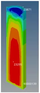 Fig 2. Simulated battery to generate training data. Training and testing points are indicated.
There is a preprocessing option built in, but we will assume that the data is ready to be used for training. Once the training dataset is organized in a spreadsheet or matrix, it can easily be imported into the romAI interface. Next, we will need to select a folder to save the model and give it a name. The tool can recognize the column headers as data labels, which we can then select as inputs, outputs, and states. Figure 3 below shows the first three sections of the GUI that allow us to complete these first steps of the neural network training process.
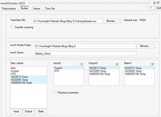 Fig 3. romAI GUI for preparing training dataset.
After initializing the data and the setup on our machine, we can begin to actually define the structure of the network. Again, the romAI interface allows us to quickly and easily choose these architectural parameters without extensive knowledge of the code behind the scenes. For this example, we will create a relatively simple non-linear model. Between the rectified linear unit (relu) and the hyperbolic tangent (tanh) activation functions, we will choose tanh. We will also increase the number of hidden layers from two, the default, to three, with each layer having 20 neurons. These selected options can be seen in Figure 4.
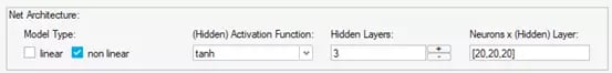 Fig 4. romAI GUI for defining network architecture.
Finally, the last step before training the model is to set up the training parameters. There are of course the straightforward ones, such as number of epochs (the number of “training cycles”), the test split ratio (how much of the data is used to test the model each epoch), and the learning rate (a measure of how much the model adjusts each epoch). We can tune the model even more by normalizing the output, which helps to train faster and more accurately. The last important piece of the puzzle is the optional early stopping. It is a good idea to set this up on most models, as it allows you to train faster and avoid “over-fitting” the model. Over-fitting will cause the model to lose its ability to extrapolate to datasets it has never “seen” before, and it may only ever work on the data with which it was trained. Figure 5 shows the values for each of the previously discussed parameters I used for this model. There are a few others that I did not mention, but the help window within the GUI offers detailed explanations for each one.
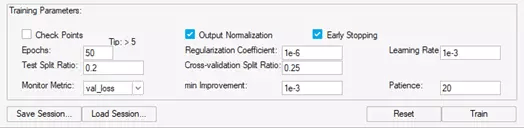 Fig 5. romAI GUI for defining training parameters.
After training the model, we have a few methods to see how it performs on the “Viewer” tab of the GUI. First, we can view the loss-vs-epoch data. This will show us how well the model adapted to the training data each epoch, as well as how well it performed on model validation data (which was determined in the test split ratio we defined earlier). In Figure 6, we can also see that the model only needed 28 epochs before the early stopping caused it to complete before the maximum of 50 epochs.
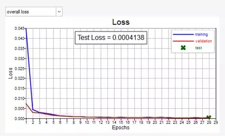 Fig 6. Overall loss vs epoch of model with early stopping
On this same tab, we can view the accuracy of the model on a new test set of data that it has not seen before. This test set is very similar to the training dataset, with the key difference of having a new HTC that was not present during training. Figure 7 shows the accuracy check of the predicted vs true (target) temperatures in the middle of the battery (T23295). With an R2 value of 0.9978, we can safely assume that the model does a pretty good job of predicting the temperature at this point.
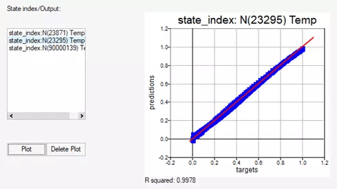 Fig 7. Predictions vs targets; accuracy of model at given point.
The final key performance indicator can be seen on the “Time Sim” tab, which will show us the temperature at one of the given points over time within the battery. Again, I will show the curves for the middle of the battery in Figure 8, which shows just how similar the model and true dataset are over the discharging cycle of the battery.
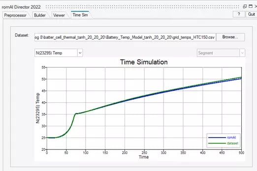 Fig 8. Time simulation of model at given point on new test dataset.
And just like that, we have taken a set of measurements and turned it into a powerful and valuable neural network with only a few clicks within Altair Compose and romAI. There are a few results that I did not show, such as the validation for other points during training and the time-simulation results for the other points on the battery with the new HTC during testing. This dataset comes pre-loaded with romAI, though, so feel free to open it up and give it a try on your own machine. Play around with the model architecture and training parameters to see if you can improve on the network we built in this example. As always, feel free to reach out to us with any questions or comments, and remember to check out our blog and YouTube page routinely for new content like this!