
TrueInsight
Siemens/Altair Channel Partner
Menu


Solving and Visualizing Differential Equations in Altair Compose
Altair Compose can be used for many applications to simplify your workflow. In this blog, Fletcher Turner walks through solving differential equations.
Although many software suites and engineering tools are capable of automatically applying numerical solutions to differential equations “behind the scenes,” it could be valuable in many instances to find a preliminary solution yourself. For example, you may want to start designing based on simpler models or equations before diving into the details of a more fine-tuned simulation of an entire system. Or perhaps you are prototyping and have wider tolerances that don’t necessitate a more complex model in your current stage of design. Whatever the reason, it can be helpful to solve differential equations “manually,” which is where Altair Compose comes in to save the day. I say “manually” because, while the software still does the bulk of the work for you, it requires a little more user input on the “math” side than designing geometry and adding larger system definitions.
Using the open matrix language (OML) of Compose’s code-based interface, we can solve a wide variety of differential equations. There are a number of prebuilt ordinary differential equation (ODE) solvers within the tool, which allow users to choose the numerical method used to solve the problems of interest. As an example, I will walk through the process of setting up and solver one of the telegrapher’s equations in Compose.
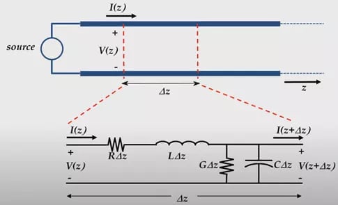
Fig 1: Transmission line lumped-element model.
For readers unfamiliar with these equations, they are used to find the voltage and current on a transmission line at a specific location and time. Fig 1 above shows the basic model that represents such a system, where R, L, G, and C are unit resistance, unit inductance, unit conductance to ground, and unit capacitance to ground, respectively. The equations use the lumped-element approach to analyze the entire system over discrete units defined with a length of Δz.
For the purpose of this blog, I will only continue with the analysis of the voltage at a given time and z location along the transmission line. With some knowledge of circuits and calculus, the following expressions can be derived to model the voltage of interest. Equation 1 shows the full equation in terms of R, L, G, and C, while Equation 2 shows the simplified representation of the same equations, where a, b, and c are condensed coefficients in place of the physical circuit parameters.
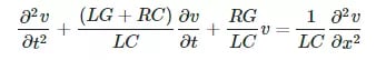
Equ. 1: Telegrapher’s Equation for Voltage.![]()
Equ. 2: Condensed differential equation for OML input.
The rest of the problem can now be addressed in Compose. The basic first steps are to define our discretized transmission line and differential matrix. From here, we can define the actual input voltage, which will kept simple as cos(x), and necessary boundary conditions. There are several options available to further refine the approach to the problem; in this case, we just set the max step of the solver equal to Δz, so the automatically adjusted solver step size does not exceed the finite length of each segment in the numerical discretization of the model. Fig 2 below shows a snippet of the code used to set up the solution.
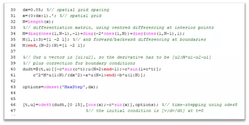
Fig. 2: Example of OML code to solve the problem.
In Fig 2, you will also notice the last line is where we actually tell Compose to solve the differential equation using the built-in function ode45, which uses an adaptive Runge-Kutta algorithm. As I mentioned, there are other options for this function, so feel free to browse Altair’s extensive documentation to find the solver right for you!
Our answers are provided in a matrix that represents the voltage at all combinations of discretized times and lengths. Compose provides powerful graphing tools to visualize these results in a number of ways. For instance, we might be interested in comparing the voltage signal at the input and the output of the transmission line over time. Fig 3 shows exactly these results. Using the further functionality of Compose, we can measure that there was a reduction in amplitude of approximately 5.6% and a phase shift of approximately 217° (or -143°).
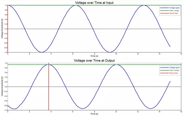
Fig. 3: Voltage signals as function of time at transmission line input and output.
We can also use Compose to animate our results for a deeper dive into the solution of our problem. Fig 4 below shows the animated voltage as a function of time over the length of the transmission line. By that, I mean that the x-axis represents the physical length of the entire model, while the y-axis still represents the voltage. The only difference here is the animation shows the signal changing over time, which lets us see the live changes in the voltage signal over the length of the transmission line.
Fig. 4: Voltage signal over length of the transmission line animated through time.
This approach could be very valuable when it comes to the initial design stages of a problem, where you are more interested in a ‘coarser’ model of your system before you take the time to design and simulate in greater detail (hopefully using another Altair product!).
As always, if you have any questions, comments, or suggestions, please do not hesitate to reach out to us at TrueInsight!