Leveraging Simcenter Hyperstudy & PSIM Part 2: From Integration to Optimization

In a previous blog post and video, we discussed how to successfully integrate Simcenter PSIM, the frontrunning tool of circuit design and analysis, into Simcenter Hyperstudy, an industry leader in design exploration and optimization. One of the primary benefits of Hyperstudy is providing the ability for users to simulate and compare a wide range of studies for a given design, all without the need to manually iterate. With these tools working in tandem, it becomes possible for engineers to rapidly simulate, analyze, and optimize power electronics, motor drives, and circuit schematics in a range of other applications. Let’s take a closer look at some of the specific options available once the connection is established between these software solutions.

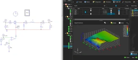
Fig 1. View of project in PSIM (left) and Hyperstudy (right).

As a reminder, this analysis is related to a buck converter with an input of 11.1 V and a desired output of 5.55 V. The resistance, capacitance, and inductance of the ideal passive elements are the parametric values that can be tuned, in addition to the duty cycle of the switching signal.

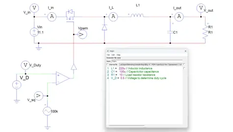
Fig 2. Circuit schematic in PSIM to be optimized.

Optimization Setup

Before users can run this type of optimization in Hyperstudy, a few basic steps are required to customize the analysis to your needs. Much of the information related to the model definition (the schematic, parameters, nominal values, etc.) is automatically populated if you create the Optimization using the setup outlined in the previous blog post as the starting definition.

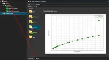
Fig 3. Creating an Optimization from our existing model in Hyperstudy.

These values will automatically match the values provided in the initial setup, but they can be changed if desired. For this example, we will keep the nominal inputs, parameter bounds, and output responses (overshoot percentage and steady state voltage) as before.

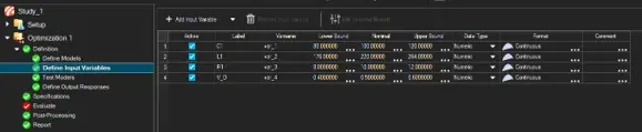
Fig 4. Parameter ranges in Hyperstudy.

For our output responses, we can also now define goals and constraints. For this simple buck converter, we will provide a goal to minimize the overshoot percentage. We can also define multiple constraints to the steady state voltage value; we will use Steady Stage ≥ 5.5V and Steady Sate ≤ 5.6 V to attempt to keep the output ripple within approximately ±1%.

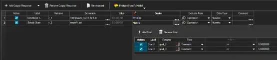
Fig 5. Defining optimization goals and constraints in Hyperstudy.

Running the Optimization

Once the model has been defined, the parameter ranges are determined, and the goals have been established, you are almost ready to run your optimization. The final steps are to choose exactly how Hyperstudy will perform the optimization. These options include localized and global gradient searches, single and multi-objective handling, and reliability analysis.

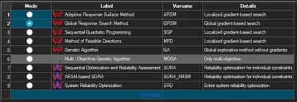
Fig 6. Optimization methods available in Hyperstudy.

For this example, we will choose the Global Response Search method; we can also choose the number of iterations and failed evaluation handling. These give instructions on how many simulations to perform and how to handle results that do not align with the desired optimization boundaries, respectively.

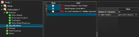
Fig 7. Choosing Optimization settings in Hyperstudy.

Hyperstudy also gives us the ability to define a number of simulations to run simultaneously, allowing us to get our results even more rapidly. Based on your hardware available, you can utilize parallel execution to evaluate multiple designs at the same time instead of waiting for each run to finish sequentially. Now we are ready to run the optimization!

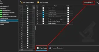
Fig 8. Setting parallel tasks and launching optimization in Hyperstudy.

Optimization Post-Processing

Now that the optimization is complete, Hyperstudy gives us many options to analyze the results and extract valuable information. First, we can review a summary of the combinations of parameters that were searched and tested, in addition to the outputs of each simulation and how they performed against the constraints and goals. This table also includes the resulting optimal values based on the settings we have defined.

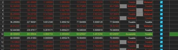
Fig 9. Summarized results in Hyperstudy with optimal parameters highlighted in green.

We can also display a variety of results, such as iteration plots, scatter plots, and other tools to see how the optimization arrived at its results. These outputs also allow us to visualize which parameters had the most significant impact on various measurements or goals. For example, we can display a 3D plot showcasing the combination of effects from various inputs, and we can generate a trade-off plot, comparing the results of both output metrics.

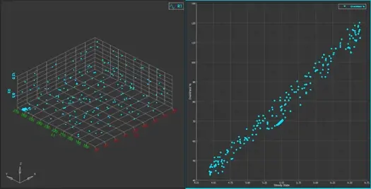
Fig 10. 3D Scatter Plot and Output Trade-Off Plot Hyperstudy.

We can also test the new optimized values back in the original PSIM software to see the full scope of the results.

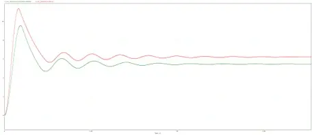
Fig 11. Optimized results (green) verified against non-optimal results (red) in PSIM.

This is just the beginning of what’s possible when you combine the circuit analysis capabilities of Simcenter PSIM with the design exploration and optimization strengths of Simcenter Hyperstudy. Perhaps you would like to take this a step further on your end and add a closed loop controller, which can also be optimized in Hyperstudy. Be sure to continue checking out these blogs for more information about this powerful cooperation between these tools, and remember to subscribe to our YouTube channel for even more content like this. If you have any specific questions about either of these tools, how they work together, or how other tools we offer may benefit you, please contact us directly!