Optimizing a Design in Altair FEKO

Optimizing a Design in Altair FEKO

I’m sure many engineers are very familiar with the term “ideal” when it comes to designing and analyzing systems or models in their various disciplines. I know it was always frustrating when I would learn about a new subject in my electrical engineering courses, and the equations never really matched the real world, because they assume that every component and condition is “ideal.” Yes, these equations and textbook models can get you close to your goal, but sometimes engineers need more accurate results than a ballpark estimate. That is where the power of optimization comes in within Altair FEKO. Within the software, there is an additional tool called OPTFEKO, that will allow you to fine-tune your models to perform closer to your real-world goals than the standard design equations can get you. 

“What is OPTFEKO?” is a questions many users may have, so I’ll run through some of the basic properties before I jump into an example. OPTFEKO is a powerful optimization tool that can be configured under the “Request” ribbon of FEKO. With variables defined in the model, you can establish parameters, which specify a range that these variables can change within with optional constraints relating variables to each other (for example, you want to ensure that one variable is always larger than another). Additionally, you can add goal functions that tell the optimizer how you want certain outputs to behave; if there are multiple goals, you can also define relative weights based on which goals are more important. And most importantly, you have the option of choosing between several optimization methods, including particle swarm, genetic algorithm, and grid search, with various customizations available to each one.

To demonstrate some of OPTFEKO’s capabilities, I’ll walk through a simple microstrip example. I used the various tools and equations available to engineers to generate some basic design parameters for a microstrip line to operate at 2.5 GHz with an FR4 substrate and gold conductor. 

 
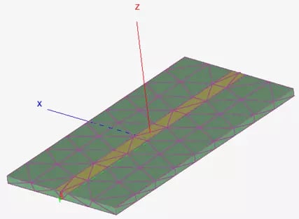
Fig 1: Simple Microstrip line to be optimized.

After creating the model shown in Fig 1, establishing an S-Parameter configuration, defining a frequency range, and running the simulation, I can view the results in POSTFEKO. Fig 2 shows that the design works well,  but at 2 GHz rather than 2.5 GHz. For some applications, this might be good enough, but for the sake of demonstration, I will assume that I need a design that performs like this much closer to 2.5 GHz. 
 

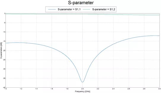
Fig 2: Initial S-Parameters of model.

To accomplish this task in using OPTFEKO, there are a few requirements. First, I have to add a Search to the model. Fig 3 shows the optimization task bar (located under the Request ribbon in CADFEKO), and the options available when creating a new Search. Here you can select a method, for the optimizer, define its accuracy level, and optionally provide a maximum number of iterations of optimization. 

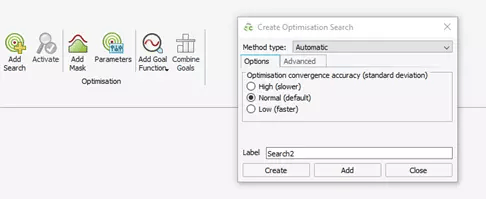
 Fig 3: Creation of Search within Optimization Tools.

Next, any values that I want to optimizer to change need to be defined as variables in FEKO. For this model, I’ve chosen the parameters related to the size of the substrate (depth, height, and width) and size of the conductor (width and thickness) to be altered during optimization. Fig 4 below shows these variables, as well as the range to which they are confined (in mm). Optionally, a starting value and grid points for each parameter can be chosen, but leaving them blank will allow the tool to automatically define grid points, and it will start at the middle value between the defined minimum and maximum. 

 
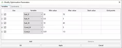
Fig 4: Definition of parameters and their respective ranges.

After telling FEKO what it can change and by how much, we’ll need to tell it what we want the results to look like, which can be accomplished by adding one or more Goal Functions. There are several types of goal functions available based on what you are trying to achieve, but in this example, we’ll stick with trying to alter the S-Parameters. Fig 5 depicts this setup, in which I have defined a goal for the magnitude of the Reflection coefficient S11 to be equal to zero (or negative infinity in dB) at 2.5 GHz, which is not possible, but it will tell FEKO to provide a model that lowers that value as much as possible, within the provided constraints. I also added another goal to ensure that the coupling coefficient between S11 and S11 is as close to 1 (or 0 dB) as possible, but I lowered the weight from 1 to 0.2. 
 

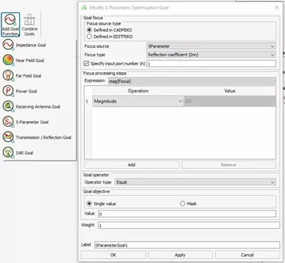
Fig 5: Reflection Coefficient Optimization Goal.

At this point, I am ready to run OPTFEKO in the Solve/Run tab. There are a few other options in optimization that I skipped over, such as adding a Mask; if we had the x-y coordinates of our desired S-Parameter plot, this would allow us to import that and define that Mask as our goal in the Goal Function, but this can be computational expensive, as it must simulate the model over a range of frequencies, rather than just one desired operating frequency. Fig 6 shows the POSTFEKO results of running the optimization. There are many datasets available here, such as performance of each output relative to the goal functions, the output of the global goal function as it attempts to reduce the error over each iteration, and any masks you may have defined. Here I have chosen to display the values of the 5 parameters we selected earlier over each iteration. Notice how they all eventually approach a steady state, as the model gets closer to the goal, and then they each terminate once there are no more significant changes in the outputs relative to the goals. 
 

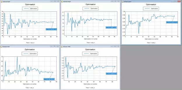
Fig 6: Progress of parameter values over the course of optimization.

From here, we can record the final values of the substrate depth, height, and width, as well as the terminal values of the conductor width and thickness. These record numbers can then be plugged back into the original model to alter the physical dimensions of the device, and we can run the solver for the new S-Parameter configuration. The results of the updated simulation are shown in Fig 7 below. Here we can clearly see that the operating frequency has shifted up, as we desired. It actually looks like our new model does even better at 2.5 GHz than the previous one did at 2 GHz! 
 

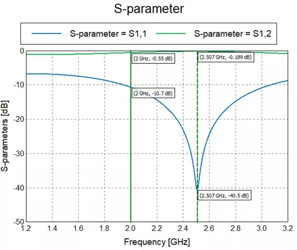
Fig 7: S-Parameter results of optimized microstrip model.

    We have successfully walked through an optimization problem in Altair FEKO. There are many more ways to go about this, and we can always get even more thorough in our setup and analysis, but I hope this overview was informative and interesting! As always, feel free to reach out with any questions or comments!