
TrueInsight
Siemens/Altair Channel Partner
Menu


Manually Tuning a PID Controller in Altair Embed
Learn how to manually tune a PID controller in Altair Embed with our step-by-step guide. Our post covers the basics of PID controllers and tuning process.
In the world of electrical engineering, control plays an integral role in device performance at multiple levels. There are countless methods of characterizing systems and designing control systems. No matter which of the approaches you use, it is extremely useful if you are able to simulate your design before you build anything in the real world. Once you have modeled you entire system, many times you will find that changes are necessary to optimize the design. Again, there are several methods available for engineers to accomplish this goal, but many of them can be tedious, such as making the change and rerunning the entire model or parameterizing the model and comparing the array of results. These workflows might be beneficial in certain applications, but other engineers could be interested in examining minor changes in real-time with real systems. This is where the power of Altair Embed can be seen.
Altair Embed is a powerful embedded systems design software with a wide range of capabilities to assist in every stage from initial design to implementation. It comes preloaded with an array of blocks including microcontroller pins, control schemes, and physical hardware. In this example, we will walk through controlling a DC motor using a basic PID controller. First, we will need to place the DC Motor block into our schematic, which is actually a system of systems on its own, with ‘smaller’ blocks inside of it to represent various parameters, such as armature resistance and, motor inertial, and back EMF. Figure 1 shows the cascading “subsystems” from the main DC Motor block to the system representation within, to yet another subsystem transfer function representation of the armature, where motor parameters can be edited. We will keep the default values, but you can enter information for whatever motor you have on hand. We can see that our inputs are the armature voltage Va and the load torque TL, and our outputs are the Speed (rad/s) and motor position An (rad). Since we are building a model around a controlling speed (we will not treat this as a servo motor, although we could if we wanted to), we will only be interested in the motor speed.
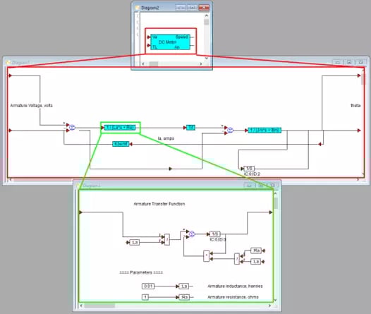
Fig 1. DC Motor block and cascading subsystems
After establishing and defining our plant, we could spend some time characterizing it and determining its transfer function, but we will skip straight to implementing a controller (you will see why shortly). Again, we can use the prebuilt PID block (pid_ctl) in Embed, but we will need to make a few minor modifications. Before we make any changes, though, we can see the two inputs: Setpoint and Feedback, as well as the one controller output signal in Figure 2. The red box shows the “zoom into” the PID Control block. In the same Figure, the two modifications we need to make are also highlighted. In the purple box, we changed the Integrator block to a Limited Integrator block, so we can apply limits and avoid ‘integral windup,’ and the in the green box, we applied a limit to the controller output to keep it between 0 and 50; this will act as the ‘voltage’ supplied to the motor in the range of 0 V to 50 V. This is a bit simplified compared to an actual motor control system, but the logic stays mostly the same.
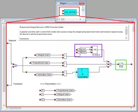
Fig 2. PID Control block and internal subsystem modifications
Now we are at the stage where we can actually begin customizing our control and plan the next design stages. There are many ways to compare results based on simulation configurations, but Embed offers a an easy-to-use tool that will let users hone in on ideal values: the slider input. Figure 3 shows a few examples of this tool that we are going to use in this simple simulation. These sliders allow users to define a range of values and the incremental change within that range. Here we have set up the proportional, integral, and derivative terms with ranges of 0-2000, 0-100000, and 0-10, respectively, each with an increment of 1%. We then connected each of these sliders to their respective variable, which allows us to use that value anywhere else in the model (including within the PID control block). Now, when we run the simulation, we can change the PID values on the fly! This will allow us to view the effectiveness of the control system with different parameters while we are running the simulation. This is why I said we could skip the normal steps of analytically finding the control values.
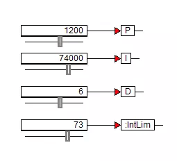
Fig 3. Slider inputs to manipulate variable values
From here, all that is left to do is finalize the setup of our simulation. Once we have the plant, control system, and feedback all connected, we can add a few more sliders with variables, and a plot to visualize our results. I added a slider for the set point so that we can change our desired motor speed from 0 to 10 rad/s, and I added a slider from 0 to 100 Nm for the Load Torque, so we can see what effect that has on the system. Plugging the variables into the plot is straightforward, and each signal will be plotted in the color of the selected plot input, allowing us to quickly identify individual curves on a plot with multiple datasets. Finally, we can set the system properties to run the simulation over a given time frame at a specific sample frequency. It is important to note that I checked the “Auto Restart” option, which will continuously restart the simulation. This allows us to see a non-stop run of the system as we change various parameters. An overview of this configuration is shown in Figure 4.
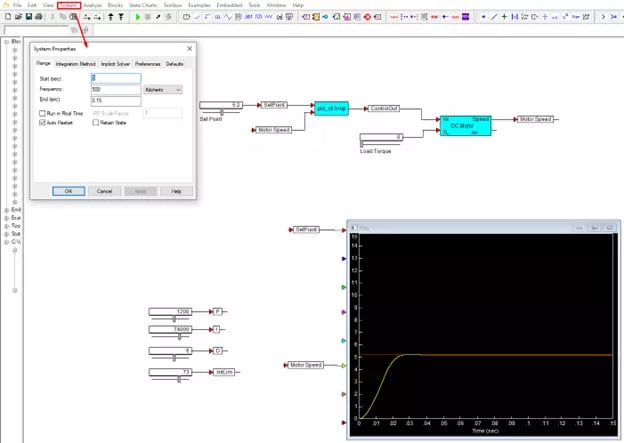
Fig 4. Simulation setup and configuration
All that is left to do now is to run the simulation and manipulate the slider values. The animation in Figure 5 below shows the set point (red) and the motor response (yellow) in a continuous loop of the first 0.15 seconds of runtime. We can see initially, when the controller is ‘off’ that the motor does not behave as desired. However, as we change the PID values, we can home in on an ideal performance. This allows us to actively see what control variables will result in certain overshoot values, settling time, and steady state error. We can also see how changing the target speed and load torque affect the performance of the overall model.
Fig 5. Running simulation and editing parameters.
From here, engineers have the option to further refine the design of the system or to add further complexity to the model in order to prepare for real-world implementation. Through this brief overview of a relatively simple example, we can begin to understand the power and versatility of Altair Embed. We have only just begun to scratch the surface of what is possible within this tool, so please feel free to reach out to us directly with any questions or comments regarding this topic! For more information on Embed and the broad suite of Altair software, please check out our other blog posts or visit our YouTube channel.