Analysis Toolboxes in Altair PSIM

Altair PSIM is the premier circuit designer and power electronics analysis software. While it allows users to lay out their circuits, define parts in any range from ideal to highly customized, simulate performance, and measure just about any voltage or current within the model, that is not all it is capable of. We will just begin to scratch the surface today as we take a look at some of the analysis toolboxes available to users with Altair PSIM: Fault Analysis, Sensitivity Analysis, and Monte Carlo Analysis.

To begin, I will use a simple buck converter to demonstrate all three of these analyses, but remember that the complexity can go up here to anything you may be designing within PSIM. Figure 1 displays the schematic of the converter, and the accompanying Table 1 shows the values for each component in the model. For this example, the nominal values for each component will never change, but for a given type of analysis, we may vary the value of one or more components. All these analysis toolboxes can be found under the “Analysis” tab within the software.

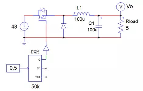Fig 1. Buck Converter Schematic

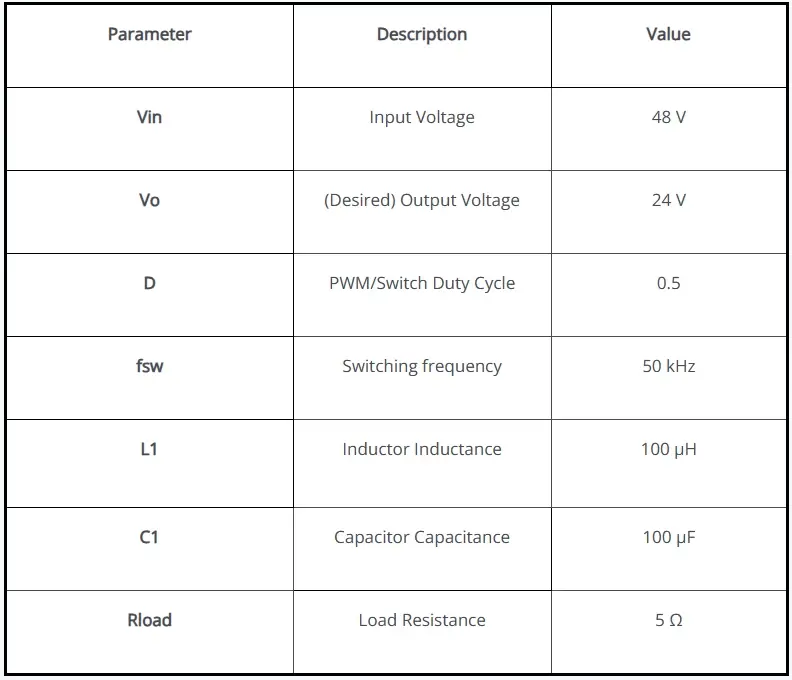
Table 1. Buck Converter nominal parameter values

Fault Analysis

The first tool we will look at is the Fault Analysis process. You can create any number of faults for any given component in the model. The fault types include short-circuits and parameter failures, where short-circuit simulates the part failing and shorting its terminals together, and parameter failure allows you to choose one or more parameters of a given part that fail and have a different value than the nominal value; for instance, if you define the On Resistance of the MOSFET as a certain value, you can examine a failure where it suddenly changes to another value. You can analyze these one at a time or in groups as a sort of “worst-case scenario.” For our example, we will examine what happens when the load (R_load) fails as a short circuit. Figure 2 shows what the “Faults” window looks like after we define this example fault.

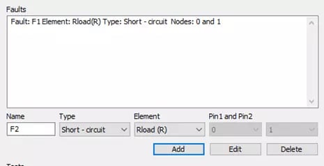Fig 2. Fault Analysis Fault Definition Panel

The next step is to determine the test we would like to perform with this fault taken into consideration. You have the option to analyze any measurement (Scope) that exists in your model, and you can select how you want to read that scope from the following: Maximum value, minimum, mean, RMS, steady state, peak to peak, and overshoot. Lastly, you can select the criteria to check for in this analysis by defining an operator (equal to, less than, or greater than) and a value. For this example, we want to see if the current through the inductor ever exceeds 50 Amps when our previously defined fault (the shorted load) occurs. Figure 3 displays this Test setup and the window that allows you to define these Tests.

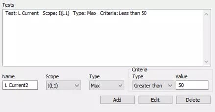Fig 3. Fault Analysis Test Definition Panel

After we have defined our Faults and Tests, we can run the analysis, and we are presented with the results shown in Figure 4 below. From here we can see that the maximum value simulated is 2.4 kA, which is well above the threshold of 50 A, so the analysis parameter “Valid?” returns as true. This lets us know that if the load were to short-circuit for whatever reason, we could expect current well above our rating of 50 A, which might lead an engineer working on this problem to reconsider the design or implement further safety measures.

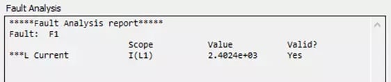Fig 4. Fault Analysis Results Panel

Sensitivity Analysis

The next tool we will examine is the Sensitivity Analysis. Using this tool, we can examine how sensitive a measurement is with respective to changing inputs or parameters. Similar to the Fault Analysis toolbox, we can define how we want certain components to behave in the Sensitivity Analysis. The difference here is that once we select a component, we can enter its nominal value and the percent variation from that value we can expect. For this example, we will vary the values of the inductor’s inductance and the capacitor’s capacitance by 5% from their nominal 100 µH and 100 µF, respectively. This configuration is seen in Figure 5.

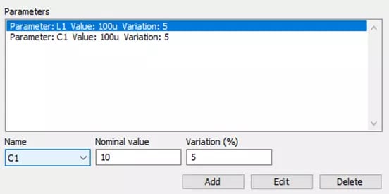Fig 5. Sensitivity Analysis Parameter Definition Panel

Again, similar to the previous analysis, we can now define what we actually want to analyze in the Outputs section of the toolbox. We can define our output as any scope within the model, and we can measure its maximum value, minimum, mean, RMS, steady state, peak to peak, or overshoot. For this example, we want to see if inductor current ripple is more sensitive to the inductor or the capacitor, so we will select the inductor current as our Scope, and the peak to peak of this measurement as our Type, as seen in Figure 6.

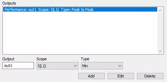Fig 6. Sensitivity Analysis Output Definition Panel

After running this analysis, we are again presented with a report of the results shown in Figure 7. This time, we see Abs Sensitivity (absolute), Rel Sensitivity (Relative), and Ranking. The sensitivity calculations give you a clear picture on how sensitive the output measurement is to changes in parameter values, and the Ranking shows which component has a larger effect, where more “+” symbols indicate a larger impact. In this example, we can see that the inductance is ranked higher, and it has significantly larger values in the sensitivities (regarding the magnitude of each category), which would be expected.

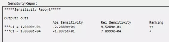Fig 7. Sensitivity Analysis Results Panel

Monte Carlo Analysis

Finally, we will walk through the Monte Carlo Analysis. With this tool, we can define a distribution of component and circuit parameter values, and then we can measure how that impacts a given output in a variety of ways. For this analysis, we can use any parameterized value in the schematic as a Monte Cristo parameter, meaning it must be defined as a variable; specifically speaking, for PSIM, the component value be equal to a variable that has not been set to a specific value yet. We can then define a distribution of values for each selected parameter using a uniform, normal, triangular, or logarithmic-normal distribution, or we can use a predefined set of discrete points. For this example, we will choose normal distributions for the capacitance and inductance, and we will define the means as 100 µF and 100 µH, respectively, while defining the standard deviations of each as 10 µF and 10 µH, respectively, as shown in Figure 8. You can input this data however you like, and it is especially helpful if you have a known distribution from the part manufacturer.

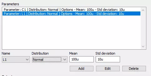Fig 8. Monte Carlo Parameter Definition Panel

Next, we can define the outputs that we would like to visualize and the measurement type for these outputs. Just like the previous two analyses, we can select any scope already defined in the model, and we can measure the maximum value, minimum, mean, RMS, steady state, peak to peak, or overshoot. Figure 9 below shows that we have set up our analysis to measure the peak to peak current through the inductor, and we have set it to run the simulation 100 times, varying the input parameters according to our previously defined distributions.

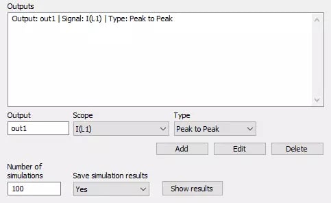Fig 9. Monte Carlo Output Definition Panel

Finally, we can view the results in a number of ways: a scatter plot of simulated values, a histogram, or a cumulative distribution function (CDF). Figures 10 and 11 show the histogram and the CDF of the Monte Cristo analysis, respectively. From the histogram, we can see the mean and standard deviation of our current ripple that we could expect if we deployed completed circuits built with components within our defined parameter distributions. The CDF of our results shows that we could expect this set of simulated circuits to have no more than 2.5A of current ripple ~70% of the time.

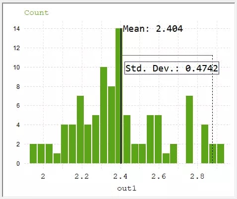Fig 10. Histogram of Monte Carlo Analysis

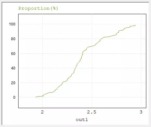          Fig 11. CDF of Monte Carlo Analysis

There are many ways to visualize, extract, and report on the resultant data of each of these analyses including, but not limited to, what we have shown and discussed here today. This example is just meant to show you what users are capable of when they start exploring more details and tools available within Altair PSIM. If you have any questions about the topics covered in this blog (or any other blog on this website), please do not hesitate to reach out directly to us. Be sure to check this website and our YouTube page regularly for new and exciting content that demonstrates the amazing extent of simulation with Altair PSIM and other Altair products.