Altair PSIM and Embed Co-Simulation

Often engineers can get used to being “siloed” into one area or subfield, and that normally means they focus all their time in one phase of the design process. When it becomes time to integrate with other systems from other specialties, much can be lost in the simplifications that must be made. These gaps in design can cause unintended consequences when all the pieces of the puzzle come together. This is where the power of co-simulation within Altair software shines. With co-simulation, we do not need to sacrifice the advantages of one software when we want to use results across various tools. To demonstrate the value of this process, we will walk through setting up and running a co-simulation with Altair PSIM and Altair Embed. 

A co-simulation between these two tools will allow us to take full advantage of the strengths of both PSIM and Embed, combining simulated results in real time. To demonstrate this process, I will use a simple but reliable example that I often find myself testing when I am learning a new tool or feature: a buck converter with a control loop. Normally, when I use the buck converter as an example, I stick strictly to an analog control scheme, which might not be very likely, depending on the application. For this example, I want to at least begin to consider the implications of designing my system with a digital controller in mind. To do this, I will need to take the delay of the digital measurement into consideration. To accomplish this goal, I will use a single pole in the feedback of the design (I will show this in greater detail when we get to that step).

Now, it might not be completely necessary to perform a co-simulation just to include a digital feedback delay, so I wanted to make this a little more complex by optimizing a controller for this type of system. This will allow us to take a deeper dive into Embed and showcase a few more beneficial aspects simulating with both tools at the same time. To begin, we will design and build a buck converter in PSIM. Figure 1 and Table 1, show the converter and values used in this example, respectively.

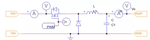Fig.1 Buck Converter

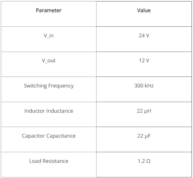
Table 1 Buck Converter Values

There are not many extra steps required to prepare a PSIM schematic for co-simulation with Embed. After designing the circuit, we will simply need to add “Link Nodes” to allow us to connect to external tools. In this case, we will use two: one In Link Node and one Out Link Node for Duty Cycle D and Output Voltage V¬¬o¬, respectively. Figure 2 below shows what this looks like in PSIM, where I have also converted most of the circuit into a subcircuit in the schematic. 

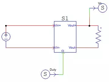Fig. 2 Buck Converter Subcircuit with Link Nodes

You will also notice that I went ahead and converted the schematic to a subcircuit. This is a relatively simple task that allows you to “tidy up” your models. To do so, simply highlight the components you wish to condense, right click, and select “Create Subcircuit.” This will save the subcircuit as a new model (that you can use anywhere in the current file or future schematics). From there, we simply need to add input and output ports, and decide where they should be visualized on the “outside view” of the subcircuit, as shown in Figure 3.

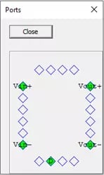Fig. 3 Subcircuit Port Definition

 Once we have our Link Nodes and our (optional) subcircuit configured, we can move over to Embed. To continue the example, I will be using the pre-made PIDTunez.vsm diagram that comes installed with Embed. This diagram will allow you to define a plant or system, and then it will optimize a PID controller, taking the measurement delay into consideration. Figure 4 below shows the overall view of the model, but I will explain a few of the most important pieces in more detail.

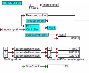Fig. 4 PID Tuning Diagram in Embed

We will start with the most obvious requirement of this model: the PID controller. This block also comes pre-made in Embed; it is named pid_ctrl.bmp by default, but we can rename the blocks by holding control and right-clicking the block to open its properties. Once we open the block by double-clicking or simply right-clicking, we can see that this is a standard PID scheme, with setpoint, feedback, error, appropriate gains, and an output, as shown in Figure 5. I will leave the finer details of how a PID controller functions for the reader, as I am sure it is mostly a review for many of you.

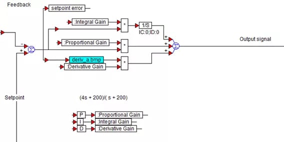Fig. 5 PID Controller in Embed

Next, the measurement is another important aspect of our diagram. When we enter this block, we can see another nested block labelled “Real Pole.” When we enter this block, we can see the block diagram representation of a single real pole, as well as the transfer function representation of this measurement delay; the transfer function is boxed in red in Figure 6. This block allows us to simulate the digital control of the plant while considering the time it takes to measure the system response.

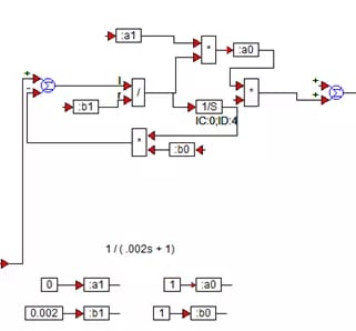Fig. 6 Real Pole to Simulate Measurement

The last pre-made part of this model that we are interested in is the “objective function,” which is where we can actually define how we want to optimize our controller. This block considers the set point error (the measured output vs the desired state) with a heavy penalty for overshooting; in this example, we are using a 10x weight for overshoot, meaning the input to the cost function will increase by a multiple of ten if the error is positive. Otherwise, we just take the unscaled error as the input. From there, we square the input, integrate it, and multiply it by 100, which will allow us to visualize the penalty on a larger scale, avoiding convergence issues. Figure 7 below shows the diagram for the cost and objective, as well as an animation of the setpoint error and objective function error over the course of the optimization.

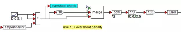Fig. 7 Objective Function and Constraint

Lastly, we are interested in defining our plant. This diagram comes loaded with an example second order transfer function, but this is where we will swap in our PSIM diagram we designed earlier. Once we double click on the “Plant” block, we can delete the “2nd order xfer func” block and add our own model. We can add the PSIMCoupler block by either searching for it using the search bar in the upper left corner, or we can find it in the data tree along the left side of Embed under Blocks > Extensions. Once we have this block in the diagram, we can navigate to the file location of our PSIM schematic and add it to our Embed model. For this specific example, I would recommend that you uncheck the “Run Simview” option, as we do not wish to open a new iteration of Simview results for each cycle of the optimization. If you wish to make any changes to the PSIM model, you also have the option to edit the schematic after importing it. This setup process is shown in Figure 8.

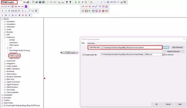
Fig. 8 Importing the PSIM Schematic via PSIMCoupler Block

Now that we have our Embed and PSIM models coming together, we just need to link the PSIMCoupler in place by connected the input (Duty Cycle) and output (Vo) to the output of the PID controller and the scaling factor, respectively; these connections are fairly intuitive and should mirror the setup of the original plant before we brought in our own. We will also need to tune a few values ourselves to allow this model to converge. First, we need to scale the output of the plant, which has a gain of 0.5 by default. We can change that to 1/24, as 0V-24V is the full operating range of the buck converter we designed initially. Next, we will need to change the input signal to have a delay of 0 (sec) and an amplitude of 0.5 (this is for a desired 12V output, so 24V/12V=0.5). The last few steps relate to setting up the parameters of the simulation and optimization itself. First we will need to open System > System Properties and set the Start at 0 (sec), the stop at 0.01 (sec), and we will need to decide a suitable simulation frequency, which was chosen to be 1 kHz in this example. Finally, we need to open System > Optimization Setup and select “Perform Optimization.” There are a few options here that I will leave as the default, but feel free to play around with them on your machine!

Now that all of that is set up, we can run the optimization. All we must do is click the Go button (the little green arrow at the top), and watch the simulation run. Figure 9 shows the process in action. We can see the plot in the lower left corner of the GIF displaying the setpoint error and objective function error, the large figure on the right shows the measured output and setpoint, and the display blocks in the middle show the values of the PID controller changing until they are optimized. Once the simulation finishes running, we have a set of controller values that we should be able to implement on the real-world system that we are modeling here (assuming it exists yet).

Fig. 9 Animation of Embed-PSIM Co-Simulation Optimization

Although this was a relatively simple example, it shows the fundamentals of just a few processes possible within the Altair suite of simulation: power electronics, control, co-simulation, and optimizations. With these tools in your own hands, the options are limitless. Feel free to pick up this project, give it a try, and even make improvements! As always, make sure to check our website and our YouTube channel for new content covering the extensive array of simulation made possible by Altair!