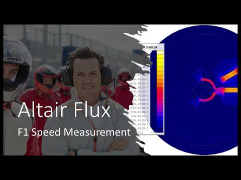
Altair Flux’s Role in Formula One

With the Formula One race in Las Vegas coming up in the very near future, I wanted to continue looking at how simulation with Altair can help engineers working on these cars or any projects like them. There is an almost endless list of aspects to ponder, design, and analyze when it comes to these incredible machines, but there is one feature that almost anyone familiar with the sport will immediately recognize as one of the most important: speed. Now, there are many aspects that determine just how fast these racecars can go, including the shape of the vehicle, the engine parameters, the tires, and so many others, but we need to be able to measure how fast the vehicle is going to tell us if any changes made to these subsystems improves the performance or not. It is also important for the drivers to have an accurate measurement of their own speed to ensure that they are racing to the best of their ability.

This is one of many places where the power of Altair Flux can be utilized. Altair Flux is the premier low-frequency electromagnetic design and analysis simulation software in the Altair suite of electrical engineering. It is primarily used for the complete simulation and optimization of rotating machines, but it can also be used for a wider range of applications, including actuators, magnetic circuit components, and power systems hardware. Today, we will take a deeper look at using the software to model a simple variable reluctance speed sensor, which could potentially be modified and implemented to measure the speed of an integral system within an F1 racecar!

The device we will be looking at will consist of one rotating cogged steel wheel with three teeth and two stationary ferrite probes with coils around each, as shown in Figure 1. The wheel will change the magnetic flux around the probes, which will create a voltage potential between them. From there, that signal could be processed and returned as a measured speed of the spinning wheel!

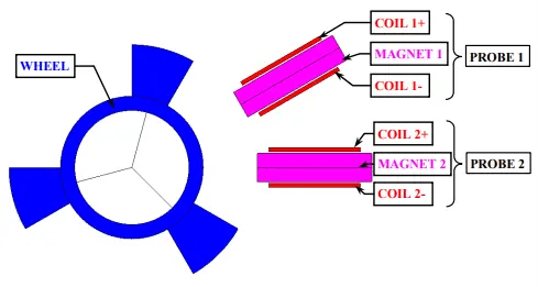Fig.1 Overview of model in this example: Cogged wheel with three teeth and two probes with coils.

The first step in this process will be to create the geometry of the device. Altair Flux contains tools for designing in 2D, 3D, and “quasi-3D” or “2.5D,” but we will be sticking to the simpler 2D design for this example. The Geometry Sketcher in the software contains many useful drawing tools, such as circles, rectangles, arcs, and segments. An additional feature that proves to be quite efficient is the ability to copy and shift already created elements. For example, in many rotating machines, there is a clear pattern that is repeated around the device; with the Sketcher, you only need to design a repeated element once, and then you can copy and rotate it appropriately. Figure 2 below shows the sketched geometry, where only one probe had to be “hand-drawn,” while the other was simply copied and translated.

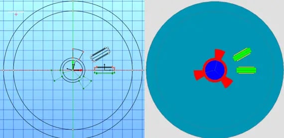Fig. 2 Sketcher Environment (left) and completed Geometry (right).

Another helpful tip to keep in mind when creating the geometry of a device is that you can create variables and parameterize them. This not only allows you to quickly make any changes necessary to the geometry, but it also helps to ensure that you are making the correct changes to the correct portions of the model. These parameters can also be used if you decide to run an optimization algorithm on the model.

Next, we will need to mesh the geometric description. Luckily, there is a powerful built-in meshing tool within Flux, which will cut down a lot of the time necessary to prepare your model for solving. Figure 3 below shows the results of the aided mesh implementation.

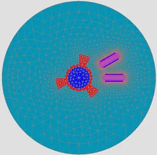Fig. 3 Geometry after automated/aided meshing.

            There are also options to further optimize the mesh for models in Flux, such as defining regions with coarser mesh to save on computation time, as well as selecting regions to have a finer mesh to more accurately measure complex areas of interest. Figure 4 shows an example of using finer mesh for the probes, coils, and the area between the probes and cogs. This will allow us to ensure we have accurate results for the most significant part of this speed sensor.

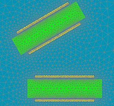Fig. 4 Close-up of refined mesh in and around probes.

One of the final steps before solving will be to assign the physics to the device. In other words, we will be defining a more fleshed out physical description of our speed sensor. This is the part of the process where we will need to tell the software what each of our previous definitions means and how each part interacts. For example, we need to tell the simulation that the wheel is a rotating component and that it is made of steel. We will need to repeat this process for each face region within our model, and the results of this can be seen in Figure 5. The image displayed shows the complete table where all geometric features are listed with all of their respective editable physical parameters. It is also worth noting that Flux has an immense catalog of electric and magnetic materials that can be implemented in any model, and each material has a provided datasheet covering vital information, such as conductive and magnetic properties.

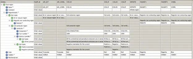Fig. 5 Table of physical definitions for regions within model.

Now we can finally define our solving scenario. For this example, we are interested in viewing the change in magnetic flux density on the probes as the cogged wheel rotates. To accomplish this, we simply need to define a scenario in which our parameter ALPHA varies within a provided range; in this model ALPHA represents the orientation of the wheel. Figure 6 shows where we can define our scenario and set ALPHA to vary by 3° per step in the range of 75° to 195°. We can define multiple scenarios as needed, depending on the specific application.

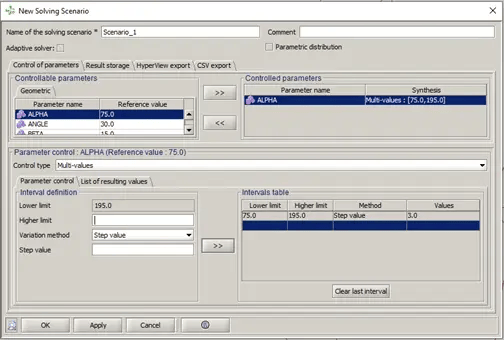Fig. 6. Creation of dynamic solving scenario.

After following the previous steps of Geometry > Mesh > Physics > Scenario, we can solve the model and move to the final stage: Post Processing. Flux offers many power Post-Processing tools, such as 2D plots, 3D plots, graphic displays, and animations. Figure 7 shows the magnetic flux density on each of the probes as ALPHA changes throughout the range defined in our solving scenario.

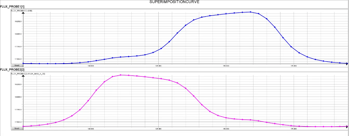Fig. 7 2D Graph of Magnetic Flux Density in probes as ALPHA varies.

We can take this a step further and show the magnetic flux density using a 3D plot, as shown in Figure 8 below. This figure shows us the measurements along the entire path of rotation as the rotation angle ALPHA changes.

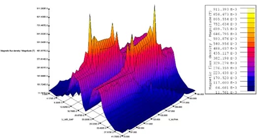Fig. 8 3D Plot of Magnetic Flux Density along path of rotation as ALPHA varies.

Finally, we can even create an animation of the changes in magnetic flux density as the wheel rotates. Figure 9 below shows the wheel changing position throughout its range of motion as well as the resultant magnetic flux density throughout the entire model.

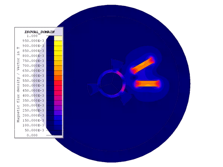Fig. 9 Animation of Magnetic Flux Density in the entire speed sensor as ALPHA varies.

This example just begins to highlight what is possible within Altair Flux. We walked through a relatively simple example displaying the key phases for this tool: Geometry > Meshing > Physics > Scenario > Solving. From there, we were able to extract any and all results of interest in a variety of formats, all while staying in the same user-friendly environment. There is an endless series of next optional steps to improve upon this model or simulate different results. You could export this to Altair HyperStudy for optimization, or you could implement this model in Altair Twin Activate as a subsystem in a larger simulation environment. See what Altair Flux can do for you by checking this blog, subscribing to our YouTube Channel, or reaching out directly to us here!